Non-target Analysis for Wastewater Treatment Evaluation
Ricardo Cunha
cunha@iuta.de29 September, 2025
Source:vignettes/articles/demo_nts.Rmd
demo_nts.RmdIntroduction
In this article we demonstrate how StreamFind can be used to evaluate ozonation of secondary wastewater effluent (i.e., effluent of the aerated biological treatment) using mass spectrometry (MS). A set of 18 mzML files are used, representing blank, influent and effluent measurements in triplicate for both positive and negative ionization modes.
basename(files) [1] "01_tof_ww_is_neg_blank-r001.mzML"
[2] "01_tof_ww_is_neg_blank-r002.mzML"
[3] "01_tof_ww_is_neg_blank-r003.mzML"
[4] "01_tof_ww_is_pos_blank-r001.mzML"
[5] "01_tof_ww_is_pos_blank-r002.mzML"
[6] "01_tof_ww_is_pos_blank-r003.mzML"
[7] "02_tof_ww_is_neg_influent-r001.mzML"
[8] "02_tof_ww_is_neg_influent-r002.mzML"
[9] "02_tof_ww_is_neg_influent-r003.mzML"
[10] "02_tof_ww_is_pos_influent-r001.mzML"
[11] "02_tof_ww_is_pos_influent-r002.mzML"
[12] "02_tof_ww_is_pos_influent-r003.mzML"
[13] "03_tof_ww_is_neg_o3sw_effluent-r001.mzML"
[14] "03_tof_ww_is_neg_o3sw_effluent-r002.mzML"
[15] "03_tof_ww_is_neg_o3sw_effluent-r003.mzML"
[16] "03_tof_ww_is_pos_o3sw_effluent-r001.mzML"
[17] "03_tof_ww_is_pos_o3sw_effluent-r002.mzML"
[18] "03_tof_ww_is_pos_o3sw_effluent-r003.mzML"The showcase will use the StreamFind MassSpecEngine, which encapsulates all tools required for parsing, storing, processing and visualizing MS data. Note that not all methods/functions will be shown, as the demonstration focuses of the workflow to assess wastewater treatment. Other processing methods for MS data are available in the StreamFind package and can be found in the StreamFind reference documentation.
MassSpecEngine
The R6 MassSpecEngine
class object is created using MassSpecEngine$new(), as
shown below. The analyses argument can be used to add the
set of ms files directly. In this demonstration, we use mzML
files. However, the original ms vendor files can also be used, but they
will be converted to mzML format using msConvert from
ProteoWizard
in the background.
# Creates a MassSpecEngine from mzML files
ms <- MassSpecEngine$new(
  metadata = list(name = "Wastewater NTA"),
  analyses = files
)
# Engine class hierarchy
class(ms)
[1] "MassSpecEngine" "Engine" "R6"
# Analyses class hierarchy
class(ms$Analyses)
[1] "MassSpecAnalyses" "Analyses" Metadata
Project metadata (e.g., name, author and description) can be added to
the MassSpecEngine$Metadata as a named list object as shown
below. The elements of the list can be anything but must have length
one.
# Adds metadata to the MassSpecEngine
ms$Metadata <- list(
  name = "Wastewater Ozonation Showcase",
  author = "Ricardo Cunha",
  description = "Demonstration project"
)

# Gets and shows the metadata
show(ms$Metadata)
name: Wastewater Ozonation Showcase
author: Ricardo Cunha
description: Demonstration project
date: 2025-09-29 15:30:45
file: NA
# Gets the date element from the Metadata
ms$Metadata$date
[1] "2025-09-29 15:30:45"Replicates and blanks
The analysis replicate names and the associated blank replicate name
can be amended in the MassSpecEngine, as shown below.
Alternatively, a data.frame with column names
file, replicate and blank could be added as
the analyses argument in
MassSpecEngine$new(analyses = files) to have directly the
replicate and blank replicate names assigned (more details here).
# Character vector with analysis replicate names
rpls <- c(
  rep("blank_neg", 3),
  rep("blank_pos", 3),
  rep("influent_neg", 3),
  rep("influent_pos", 3),
  rep("effluent_neg", 3),
  rep("effluent_pos", 3)
)

# Character vector with associated blank replicate names
# Note that the order should match the respective replicate
blks <- c(
  rep("blank_neg", 3),
  rep("blank_pos", 3),
  rep("blank_neg", 3),
  rep("blank_pos", 3),
  rep("blank_neg", 3),
  rep("blank_pos", 3)
)

# Amends replicate and blank names
ms$Analyses <- set_replicate_names(ms$Analyses, rpls)
ms$Analyses <- set_blank_names(ms$Analyses, blks)

# Replicates and blanks were amended
DT::datatable(
  info(ms$Analyses)
)
ProcessingStep
Data processing is performed by steps according to
ProcessingStep objects. ProcessingStep class objects
are obtained via the respective [Engine type]Method_[method name]_[algorithm name]
constructor functions, attributing the respective subclass. Below we
obtain the ProcessingStep for the method
FindFeatures using the algorithm openms. The
parameters can be changed via the constructor arguments. Documentation
for each ProcessingStep subclass can be found in the StreamFind
reference documentation.
# Gets ProcessingStep for finding features using the openms algorithm
ffs <- MassSpecMethod_FindFeatures_openms(
  noiseThrInt = 1000,
  chromSNR = 3,
  chromFWHM = 7,
  mzPPM = 15,
  reEstimateMTSD = TRUE,
  traceTermCriterion = "sample_rate",
  traceTermOutliers = 5,
  minSampleRate = 1,
  minTraceLength = 4,
  maxTraceLength = 70,
  widthFiltering = "fixed",
  minFWHM = 4,
  maxFWHM = 35,
  traceSNRFiltering = TRUE,
  localRTRange = 0,
  localMZRange = 0,
  isotopeFilteringModel = "none",
  MZScoring13C = FALSE,
  useSmoothedInts = FALSE,
  intSearchRTWindow = 3,
  useFFMIntensities = FALSE,
  verbose = FALSE
)

# Prints in console the details of the ProcessingStep
show(ffs)
 MassSpecMethod_FindFeatures_openms
 type         MassSpec
 method       FindFeatures
 required     NA
 algorithm    openms
 input_class  NA
 output_class MassSpecResults_NonTargetAnalysis
 version      0.3.0
 software     openms
 developer    Oliver Kohlbacher
 contact      oliver.kohlbacher@uni-tuebingen.de
 link         https://openms.de/
 doi          https://doi.org/10.1038/nmeth.3959

 parameters:
  -  noiseThrInt 1000
  -  chromSNR 3
  -  chromFWHM 7
  -  mzPPM 15
  -  reEstimateMTSD TRUE
  -  traceTermCriterion sample_rate
  -  traceTermOutliers 5
  -  minSampleRate 1
  -  minTraceLength 4
  -  maxTraceLength 70
  -  widthFiltering fixed
  -  minFWHM 4
  -  maxFWHM 35
  -  traceSNRFiltering TRUE
  -  localRTRange 0
  -  localMZRange 0
  -  isotopeFilteringModel none
  -  MZScoring13C FALSE
  -  useSmoothedInts FALSE
  -  intSearchRTWindow 3
  -  useFFMIntensities FALSE
  -  verbose FALSE
# Creates an ordered list with all processing steps for the MS data
workflow <- list(
  # Find features using the openms algorithm, created above
  ffs,

  # Annotation of natural isotopes and adducts
  MassSpecMethod_AnnotateFeatures_StreamFind(
    rtWindowAlignment = 0.3,
    maxIsotopes = 8,
    maxCharge = 2,
    maxGaps = 1
  ),

  # Excludes annotated isotopes and adducts
  MassSpecMethod_FilterFeatures_StreamFind(
    excludeIsotopes = TRUE,
    excludeAdducts = TRUE
  ),

  # Grouping features across analyses
  MassSpecMethod_GroupFeatures_openms(
    rtalign = FALSE,
    QT = FALSE,
    maxAlignRT = 5,
    maxAlignMZ = 0.008,
    maxGroupRT = 5,
    maxGroupMZ = 0.008,
    verbose = FALSE
  ),

  # Filter feature groups with maximum intensity below 5000 counts
  MassSpecMethod_FilterFeatures_StreamFind(
    minIntensity = 3000
  ),

  # Fill features with missing data
  # Reduces false negatives
  MassSpecMethod_FillFeatures_StreamFind(
    withinReplicate = FALSE,
    rtExpand = 2,
    mzExpand = 0.0005,
    minTracesIntensity = 1000,
    minNumberTraces = 6,
    baseCut = 0.3,
    minSignalToNoiseRatio = 3,
    minGaussianFit = 0.2
  ),

  # Calculate quality metrics for each feature
  MassSpecMethod_CalculateFeaturesQuality_StreamFind(
    filtered = FALSE,
    rtExpand = 2,
    mzExpand = 0.0005,
    minTracesIntensity = 1000,
    minNumberTraces = 6,
    baseCut = 0
  ),

  # Filter features based on minimum signal-to-noise ratio (s/n)
  # The s/n is calculated using the CalculateFeaturesQuality method
  MassSpecMethod_FilterFeatures_StreamFind(
    minSnRatio = 5
  ),

  # Filter features using other parameters via the patRoon package
  MassSpecMethod_FilterFeatures_patRoon(
    maxReplicateIntRSD = 40,
    blankThreshold = 5,
    absMinReplicateAbundance = 3
  ),

  # Finds internal standards in the MS data
  # db_is is a data.table with the
  # name, mass and expected retention time of
  # spiked internal standards, as shown below
  MassSpecMethod_FindInternalStandards_StreamFind(
    database = db_is,
    ppm = 8,
    sec = 10
  ),

  # Corrects matrix suppression using the TiChri method from
  # 10.1021/acs.analchem.1c00357 to better compare influent and effluent
  MassSpecMethod_CorrectMatrixSuppression_TiChri(
    mpRtWindow = 10,
    istdAssignment = "range",
    istdRtWindow = 50,
    istdN = 2
  ),

  # Loads MS1 for features not filtered
  MassSpecMethod_LoadFeaturesMS1_StreamFind(
    filtered = FALSE
  ),

  # Loads MS2 for features not filtered
  MassSpecMethod_LoadFeaturesMS2_StreamFind(
    filtered = FALSE
  ),

  # Loads feature extracted ion chromatograms (EIC)
  MassSpecMethod_LoadFeaturesEIC_StreamFind(
    filtered = FALSE
  ),

  # Performs suspect screening using the StreamFind algorithm
  # db_with_ms2 is a database with suspect chemical standards
  # includes MS2 data (i.e., fragmentation pattern) from standards
  MassSpecMethod_SuspectScreening_StreamFind(
    database = db_with_ms2,
    ppm = 10,
    sec = 15,
    ppmMS2 = 10,
    minFragments = 3
  )
)
Then, the list can be added to the MassSpecEngine. Note that the order will matter when the workflow is applied!
# Conversion of list to Workflow object with validation
workflow <- Workflow(workflow)

# Adds the workflow to the engine. The order matters!
ms$Workflow <- workflow

# Printing the data processing workflow
show(ms$Workflow)1: FindFeatures (openms)
2: AnnotateFeatures (StreamFind)
3: FilterFeatures (StreamFind)
4: GroupFeatures (openms)
5: FilterFeatures (StreamFind)
6: FillFeatures (StreamFind)
7: CalculateFeaturesQuality (StreamFind)
8: FilterFeatures (StreamFind)
9: FilterFeatures (patRoon)
10: FindInternalStandards (StreamFind)
11: CorrectMatrixSuppression (TiChri)
12: LoadFeaturesMS1 (StreamFind)
13: LoadFeaturesMS2 (StreamFind)
14: LoadFeaturesEIC (StreamFind)
15: SuspectScreening (StreamFind)
run_workflow()
The Workflow can be applied by run_workflow(),
as demonstrated below. Note that with run_workflow(), the
processing modules are applied with the same order as they were
added.
# Runs all ProcessingStep added
ms$run_workflow()
Results
The created features and feature groups can be inspected as
data.table objects or plotted by dedicated methods of the
MassSpecResults_NonTargetAnalysis
class. Internally, the MassSpecEngine stores the results in the
results list of the MassSpecAnalyses
object, which can be accessed with
MassSpecEngine$Results$MassSpecResults_NonTargetAnalysis as
shown below. The MassSpecResults_NonTargetAnalysis object can
be used for advanced operations, such as exporting the results to a
database or other formats or use the native objects from other packages
(e.g., patRoon) as
we demonstrate further in this article.
# Accessing the MassSpecResults_NonTargetAnalysis from the Engine$Results
nts <- ms$Results$MassSpecResults_NonTargetAnalysis

class(nts)
[1] "MassSpecResults_NonTargetAnalysis" "Results"
data.table objects
The features and feature groups can be obtained as
data.table with the get_features() and
get_groups() methods. The methods also allow to look for
specific features/feature groups using mass, mass-to-charge ratio,
retention time and drift time targets, as show below for a small set of
compound targets where mass and retention time expected values are
known. Note that drift time is only applicable for MS data with ion
mobility separation.
DT::datatable(db)
# Compounds are searched by monoisotopic mass and retention time
# ppm and sec set the mass (im ppm) and time (in seconds) allowed deviation, respectively
# average applies a mean to the intensities in each analysis replicate group
DT::datatable(
  get_groups(
    nts,
    mass = db,
    ppm = 10,
    sec = 15,
    average = TRUE
  )
)
Already by inspection of the data.table, it is possible
to see compounds detected in the influent but not in the effluent (e.g.,
Carbamazepine) or compounds that are appear to be reduced during
ozonation (e.g., Metoprolol). Since positive and negative ionization
mode were combined, there are compounds that appear in both polarities
and are grouped by neutral monoisotopic mass (e.g., Candesartan and
Diclofenac).
plot_groups methods
For a better overview of the results, the method
plot_groups() or even more detailed the method
plot_groups_overview() can be used.
# set legendNames to TRUE for using the names in db as legend
plot_groups(
  nts,
  mass = db,
  ppm = 10,
  sec = 15,
  legendNames = TRUE
)
plot_groups_overview(
  nts,
  mass = db,
  ppm = 5,
  sec = 10,
  legendNames = TRUE
)
Filtered not removed
The FilterFeatures method was applied to filter features
according to defined conditions/thresholds. Yet, the filtered features
were not removed but just tagged as filtered. For instance, when the
method MassSpecEngine$get_groups() is run with
filtered argument set to TRUE, the filtered
features are also shown. Below, we search for the same compounds as
above but with the filtered argument set to
TRUE. Potential features from Valsartan are now returned
but were filtered due to low intensity. Note that when extracting
features based on basic parameters, i.e. mass and time, does not mean
that features are identified. The identification of features is a more
complex process and requires additional information, such as MS/MS data
as in the processing method suspect screening.
# Set filtered to TRUE for showing filtered features/feature groups
DT::datatable(
  get_groups(
    nts,
    mass = db,
    ppm = 5,
    sec = 10,
    average = TRUE,
    filtered = TRUE
  )
)
Internal Standards
The method FindInternalStandards was applied for tagging
spiked internal standards and the results can be obtained with the
dedicated method MassSpecEngine$get_internal_standards() or
plotted as a quality overview using the method
MassSpecEngine$plot_internal_standards(), as shown below.
The plot gives an overview of the mass, retention time and intensity
variance of the internal standards across the analyses in the
project.
# List of spiked internal standards
DT::datatable(db_is)
# Gets the internal standards evaluation data.table
DT::datatable(
  get_internal_standards(nts)
)
plot_internal_standards(nts)Quality control of spiked internal standards
plot_groups_profile(
  nts,
  mass = db_is,
  ppm = 8,
  sec = 10,
  filtered = TRUE,
  legendNames = TRUE
)
Internal standards profile across analyses
Components
The method AnnotateFeatures was applied to annotate the
natural isotopes and adducts into components. Implementation of
annotation for in-source fragments is planned but not yet available with
the StreamFind algorithm. The method
MassSpecEngine$get_components() can be used to search for
components, as shown below for the analysis number 11. Because the
filters excludeIsotopes and minIntensity were
applied, the isotopic features are likely filtered.
# Components of Diclofenac and Candesartan in analysis 11
components_example <- get_components(
  nts,
  analyses = 11,
  mass = db[db$name %in% c("Diclofenac", "Candesartan"), ],
  ppm = 5,
  sec = 10,
  filtered = TRUE
)

# Subset of the components data.table
DT::datatable(components_example)
The components (i.e., isotopes and adducts) can also be visualized
with the method MassSpecEngine$map_components(), as shown
below for the internal standards added to analysis 11. Note that again
the filtered argument was set to TRUE to
return also filtered features, as the internal standards were likely
excluded by blank subtraction.
map_components(
  nts,
  analyses = 11,
  mass = db_is,
  ppm = 8,
  sec = 10,
  filtered = TRUE,
  legendNames = TRUE
)
Components (i.e., isotopes and adducts) of internal standards in analysis 11
Suspects
The methods MassSpecEngine$get_suspects() and
MassSpecEngine$plot_suspects() can be used to inspect the
suspect screening results. In the plot function, a second plot is added
to compare the experimental fragmentation pattern (top) with the
fragmentation pattern of the respective reference standard (down) added
within the database. The colorBy argument can be set to
targets+replicates to legend the plot with combined keys of
suspect target names and analysis replicate names.
DT::datatable(
  get_suspects(nts)
)
plot_suspects(nts, colorBy = "targets+replicates")Methods from patRoon
The MassSpecResults_NonTargetAnalysis object holds methods to obtain
original objects from the patRoon package. For
instance, the S4 class features or
featureGroups objects can be obtained via the
get_patRoon_features method of the
MassSpecResults_NonTargetAnalysis results. The
patRoon package provides a comprehensive set of functions,
as shown below. See more information in the patRoon
reference documentation.
# Native patRoon object
fGroups <- get_patRoon_features(nts, filtered = FALSE, featureGroups = TRUE)

fGroups
A featureGroupsSet object
Hierarchy:
featureGroups
|-- featureGroupsSet
|-- featureGroupsScreeningSet
---
Object size (indication): 26.5 MB
Algorithm: openms-set
Feature groups: M236_R1236_301, M236_R1222_300, M236_R1139_302, M240_R945_325, M240_R966_329, M242_R916_347, ... (374 total)
Features: 1662 (4.4 per group)
Has normalized intensities: FALSE
Internal standards used for normalization: no
Predicted concentrations: none
Predicted toxicities: none
Analyses: 02_tof_ww_is_neg_influent-r001, 02_tof_ww_is_neg_influent-r002, 02_tof_ww_is_neg_influent-r003, 03_tof_ww_is_neg_o3sw_effluent-r001, 03_tof_ww_is_neg_o3sw_effluent-r002, 03_tof_ww_is_neg_o3sw_effluent-r003, ... (12 total)
Replicate groups: influent_neg, effluent_neg, influent_pos, effluent_pos (4 total)
Replicate groups used as blank: blank_neg, blank_pos (2 total)
Sets: negative, positive
# Using the native patRoon's plotUpSet method
patRoon::plotUpSet(fGroups)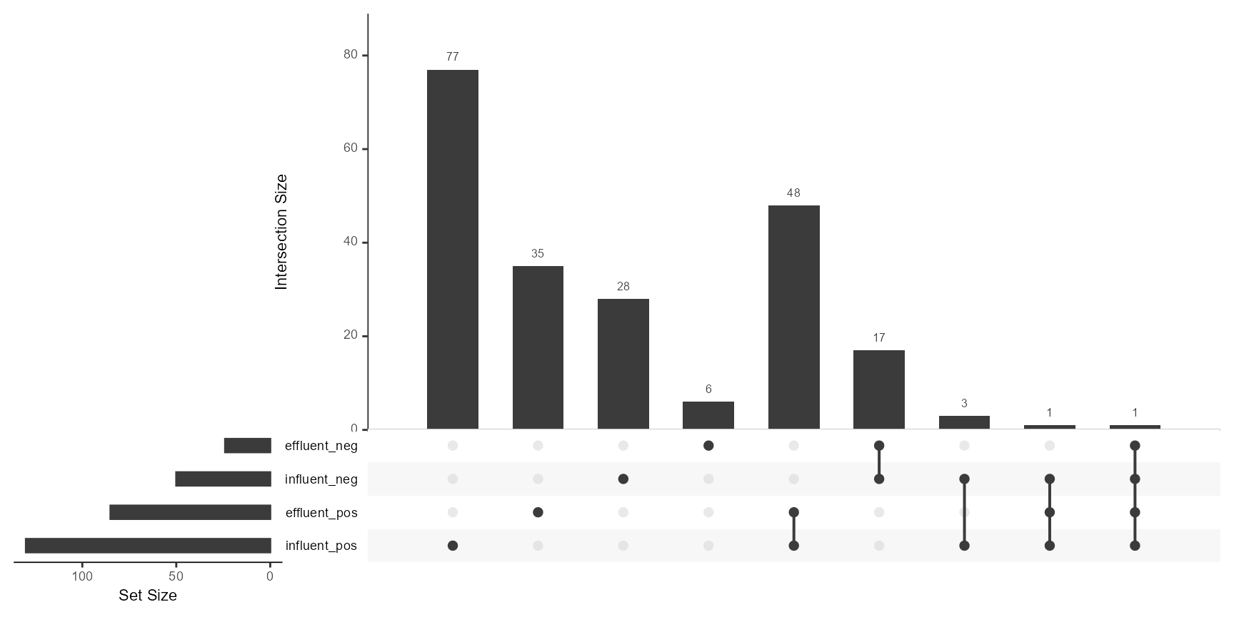
Fold-change analysis
The method get_fold_change() and correspondent
plot_fold_change() can be used to calculate and plot the
fold-change between influent and effluent samples. The method calculates
the fold-change for each feature group and replicates, as shown below.
The plot shows the fold-change for each feature group across the
replicates. The fold-change is calculated according to Bader et
al. (2017), leveraging the replicates variance to increase the
significance of the fold-change. Formation is not in the plot as no new
features were detected in the effluent of the wastewater ozonation
treatment step.
plot_fold_change(
nts,
replicatesIn = c("influent_neg", "influent_pos"),
replicatesOut = c("effluent_neg", "effluent_pos"),
filtered = FALSE,
constantThreshold = 0.5,
eliminationThreshold = 0.2,
correctIntensity = TRUE,
fillZerosWithLowerLimit = FALSE, # set to TRUE for filling zeros with lower limit argument
lowerLimit = 200,
normalized = FALSE
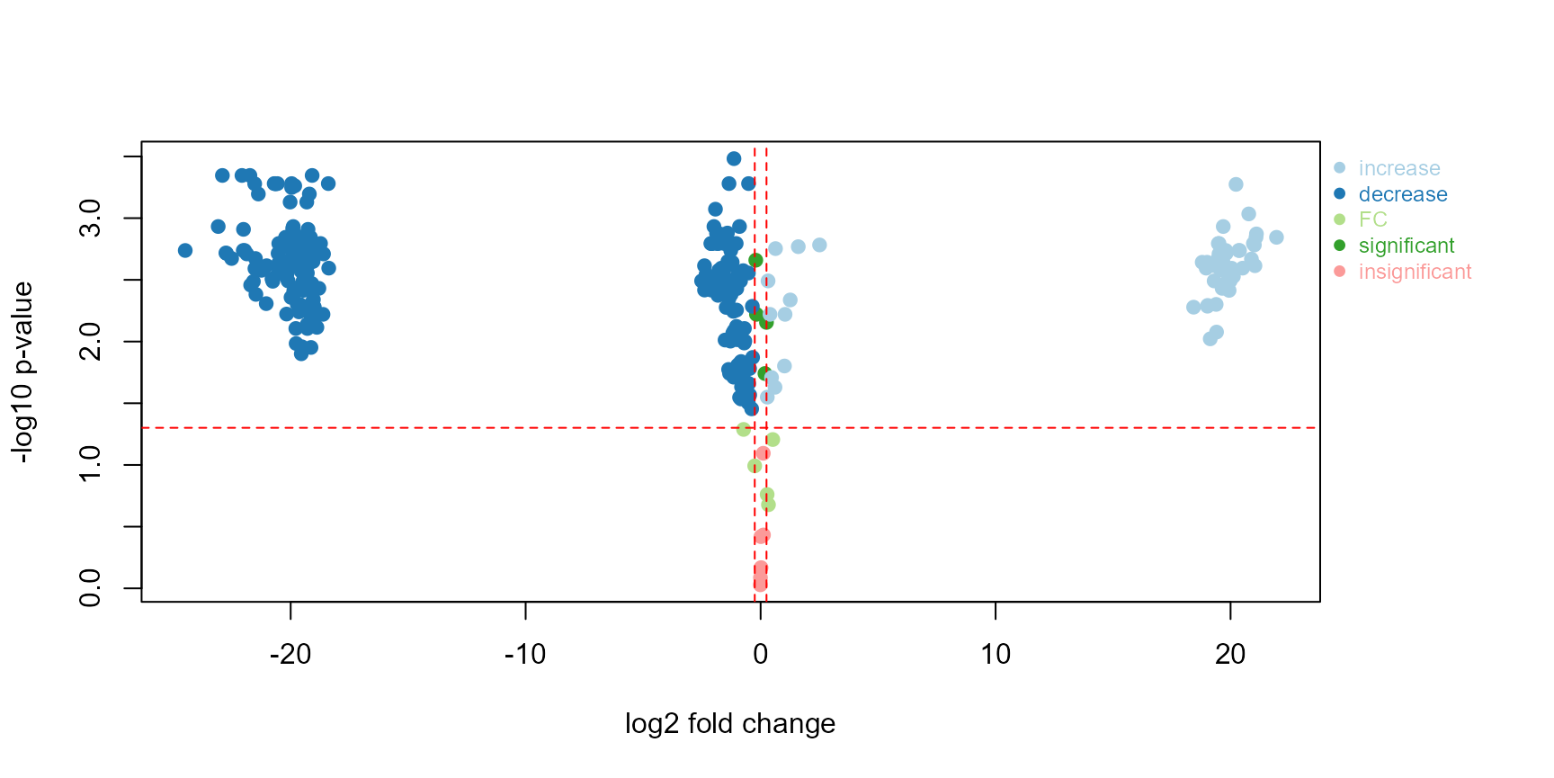
)Alternatively, the plotVolcano from patRoon can be used to
plot fold-change. For more information check the patRoon
reference documentation. Note that the function
patRoon::getFCParams is used to define the parameters for
the fold-change calculation. Below we use the default argument values,
only the in and out replicate names are set.
patRoon::plotVolcano(
  fGroups, # obtained above with get_patRoon_features
  patRoon::getFCParams(c("influent_pos", "effluent_pos"))
)
Compounds
# clone the MassSpecEngine to avoid overwriting
# R6 classes are reference classes so we need to clone to effectively copy
ms_pos <- ms$clone()

# subset with only positive analyses
ms_pos$Analyses <- ms_pos$Analyses[info(ms_pos$Analyses)$polarity == "1"]

# subsetting the Analyses, also subsets the Results
ms_pos$Results$MassSpecResults_NonTargetAnalysis$info$analysis
[1] "01_tof_ww_is_pos_blank-r001" "01_tof_ww_is_pos_blank-r002"
[3] "01_tof_ww_is_pos_blank-r003" "02_tof_ww_is_pos_influent-r001"
[5] "02_tof_ww_is_pos_influent-r002" "02_tof_ww_is_pos_influent-r003"
[7] "03_tof_ww_is_pos_o3sw_effluent-r001" "03_tof_ww_is_pos_o3sw_effluent-r002"
[9] "03_tof_ww_is_pos_o3sw_effluent-r003"
# feature groups of interest for compounds generation showncase
grs <- get_groups(nts, mass = db, ppm = 10, sec = 15)[["group"]]
grs
[1] "M236_R1079_292" "M253_R1015_479" "M267_R916_635" "M295_R1256_1105"
[5] "M325_R957_1538" "M440_R1097_2696"
# subsetting on feature groups
ms_pos$Results <- ms_pos$Results$MassSpecResults_NonTargetAnalysis[, grs]
nrow(get_groups(ms_pos$Results$MassSpecResults_NonTargetAnalysis))
[1] 6
# Applies the generates compounds using MetFrag via the patRoon package
ms_pos$run(
  MassSpecMethod_GenerateCompounds_metfrag(
    method = "CL",
    database = "comptox"
  )
)
# extract annotated compounds from the MassSpecResults_NonTargetAnalysis
DT::datatable(
  get_compounds(
    ms_pos$Results$MassSpecResults_NonTargetAnalysis
  )
)