StreamFind Get Started Guide
Ricardo Cunha
cunha@iuta.de29 September, 2025
Source:vignettes/articles/general_guide.Rmd
general_guide.RmdIntroduction
The StreamFind R package is a data agnostic data processing workflow designer. Besides data processing, the package can also be used for data management, visualization and reporting. This guide focuses on describing the general framework of StreamFind. StreamFind uses R6 classes as main interface and for project management and S3 classes for internal data handling and organization.
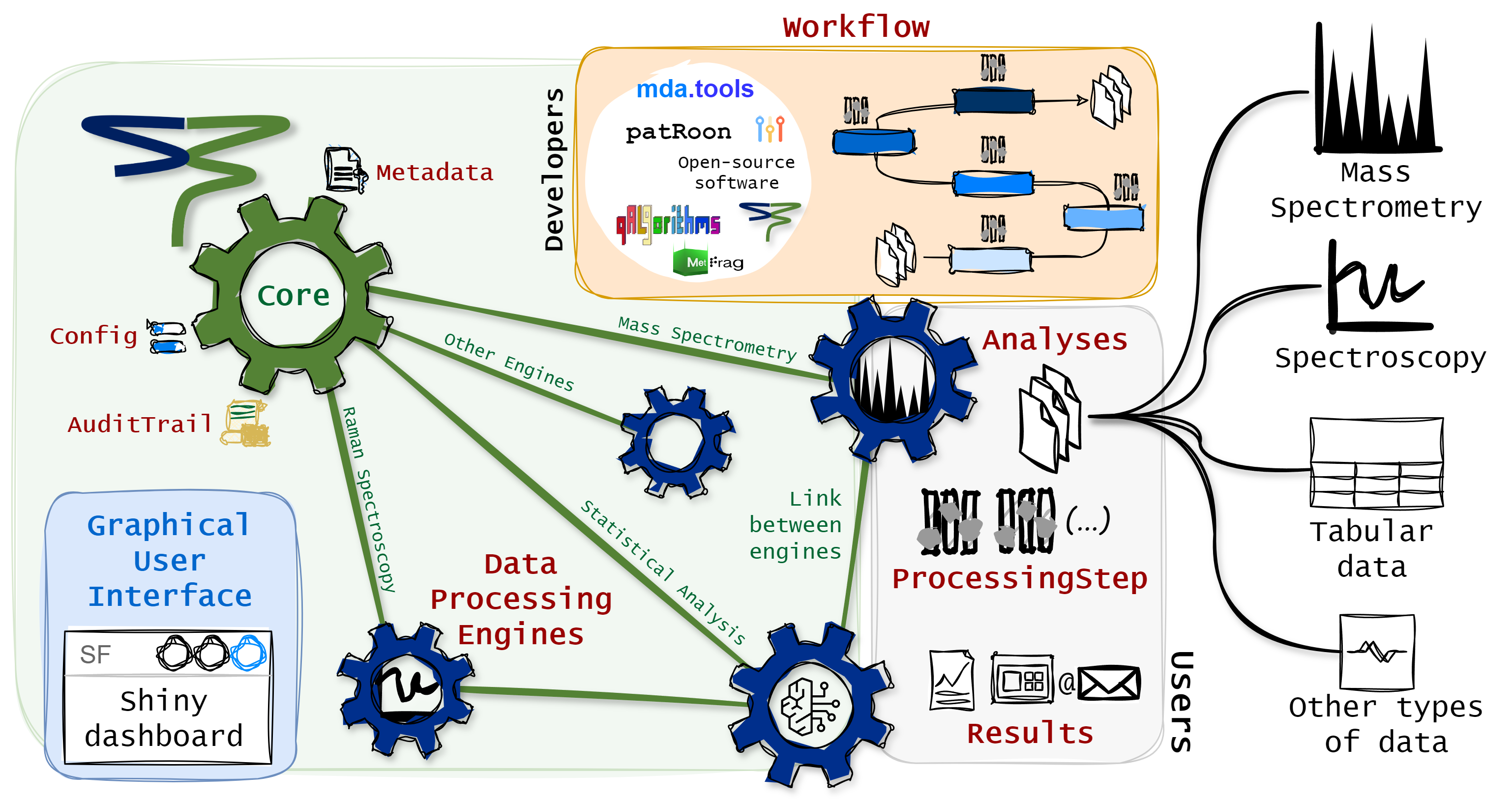
StreamFind Concept
The R6 classes have a common parent named Engine.
The Engine is the parent class of all other data specific
engines (e.g., MassSpecEngine
and RamanEngine).
The Engine holds uniform interface class objects and
functions across child data dedicated engines, such as managing the
Metadata, recording the AuditTrail and
applying the Workflow.
Internally, the Engine R6 classes use seven central S3 classes:
The Metadata is fundamentally a named list with elements
of length one, holding project information (e.g., name, author and
date). The Workflow class is an ordered list of
ProcessingStep objects, which are used to harmonize the
diversity of processing methods and algorithms available for a given
data type. The ProcessingStep class is a representation of
a processing step (i.e., algorithm to be applied to the data). The
Analyses class holds data or paths to raw data files. The
Results, which is an element of the Analyses
class, holds the results from data processing. The
AuditTrail class records any modification to the project.
The Config class holds configuration parameters for the
engines, app, etc.
Engine
Data processing engines are fundamentally used for project
management. The Engine
is the parent class of all other data specific engines (e.g. MassSpecEngine
and RamanEngine).
As parent, the Engine holds uniform functions across child
data dedicated engines (e.g. managing the Metadata,
recording the AuditTrail and applying the
Workflow).
# Creates an empty Engine.
engine <- Engine$new()

# Prints the engine.
engine
NA Engine


Metadata
name: NA
author: NA
date: 2025-09-29 15:31:32
file: NA

Workflow
empty

Analyses
empty
Note that when an empty Engine or any data specific
engine is created, required entries of Metadata are created
with default name, author, date and file. Yet, Metadata
entries can be specified directly during creation of the
Engine via the argument metadata or added to
the engine as shown in @ref(metadata). The Engine does not
directly handle data processing. Processing methods are data specific
and therefore, are used via the data dedicated engines (i.e.,
MassSpecEngine or RamanEngine). Yet, the
framework to manage the data processing workflow is implemented in the
Engine and is therefore, harmonized across engines. Users
will not directly use the Engine but it is important to
understand the background.
Metadata
The Metadata
S3 class is meant to hold project information, such as description,
location, etc. The users can add any kind of entry to a named
list. Below, a list of metadata is created and
added to the Engine for demonstration. Internally, the
list is converted to a Metadata object.
Modifying the entries in the Metadata is as modifying a
list in R and the Metadata can be accessed by
the active field Metadata in the Engine or any
other data specific engine.
# Creates a named list with project metadata.
mtd <- list(
  name = "Project Example",
  author = "Person Name",
  description = "Example of project description"
)

# Adds/updates the Metadata in the CoreEngine.
engine$Metadata <- mtd

# Show mwthod for the Metadata class.
show(engine$Metadata)
name: Project Example
author: Person Name
description: Example of project description
date: 2025-09-29 15:31:32
file: NA
# Adding a new entry to the Metadata.
engine$Metadata[["second_author"]] <- "Second Person Name"

show(engine$Metadata)
name: Project Example
author: Person Name
description: Example of project description
date: 2025-09-29 15:31:32
file: NA
second_author: Second Person Name
Workflow
A data processing workflow is represented in StreamFind by the class
Workflow.
A Workflow is an ordered list of
ProcessingStep objects. Each ProcessingStep
object is a representation of a processing step that transforms the data
according to a specific algorithm. The ProcessingStep class
is used to harmonize the diversity of processing methods and algorithms
available for a given data type.
# Constructor for a processing step.
ProcessingStep()
$type
[1] NA
$method
[1] NA
$required
[1] NA
$algorithm
[1] NA
$input_class
[1] NA
$output_class
[1] NA
$parameters
list()
$number_permitted
[1] NA
$version
[1] NA
$software
[1] NA
$developer
[1] NA
$contact
[1] NA
$link
[1] NA
$doi
[1] NA
attr(,"class")
[1] "ProcessingStep"A ProcessingStep
object must always have the data type, the processing method name,
required preceding processing methods, the name of the algorithm to be
used, the class of input and output Results objects, the
origin software, the main developer name and contact as well as a link
to further information and the DOI, when available. Lastly but not
least, the parameters, which is a flexible list of conditions to apply
the algorithm.
The ProcessingStep
is a generic parent class which delegates to child classes for specific
data processing methods and algorithms. As example, the
ProcessingStep child class for annotating features within a
non-target screening workflow using a native algorithm from StreamFind
is shown below. Each ProcessingStep child class has a
dedicated constructor method with documentation to support the usage.
Help pages for processing methods can be obtained with the native R
function ? or help() (e.g.,
help(MassSpecMethod_AnnotateFeatures_StreamFind)).
# Constructor of ProcessingStep child class for annotating features in a non-target screening workflow the constructor name gives away the engine, method and algorithm.
MassSpecMethod_AnnotateFeatures_StreamFind()
$type
[1] "MassSpec"
$method
[1] "AnnotateFeatures"
$required
[1] "FindFeatures"
$algorithm
[1] "StreamFind"
$input_class
[1] "MassSpecResults_NonTargetAnalysis"
$output_class
[1] "MassSpecResults_NonTargetAnalysis"
$parameters
$parameters$maxIsotopes
[1] 8
$parameters$maxCharge
[1] 1
$parameters$rtWindowAlignment
[1] 0.3
$parameters$maxGaps
[1] 1
$number_permitted
[1] 1
$version
[1] "0.3.0"
$software
[1] "StreamFind"
$developer
[1] "Ricardo Cunha"
$contact
[1] "cunha@iuta.de"
$link
[1] "https://odea-project.github.io/StreamFind"
$doi
[1] NA
attr(,"class")
[1] "MassSpecMethod_AnnotateFeatures_StreamFind"
[2] "ProcessingStep"
Analyses
As above mentioned, the Engine does not handle data
processing directly. The data processing is delegated to child engines.
A simple example is given below by creating a child
RamanEngine from a vector of paths to asc files
with Raman spectra. The Raman spectra are used internally to initiate a
RamanAnalyses
(child class of Analyses),
holding the raw data and any data processing Results
objects.
# Example raman .asc files.
raman_ex_files <- StreamFindData::get_raman_file_paths()

# Creates a RamanEngine with the example files.
raman <- RamanEngine$new(analyses = raman_ex_files)

# Show the engine class hierarchy.
class(raman)
[1] "RamanEngine" "Engine" "R6" Engine classes have dedicated active fields to access the major S3
classes (i.e., Metadata, Analyses,
Workflow, Results, AuditTrail and
Config). For instance, the Analyses active
field in the RamanEngine is used to access the
RamanAnalyses child class dedicated to RS. Other data
dedicated fields are also implement for data specicic engines. Consult
the documentation of the engines for more information (e.g., ?RamanEngine).
# Gets the classes of the Analyses in the RamanEngine.
class(raman$Analyses)
[1] "RamanAnalyses" "Analyses"
# S3 methods are available for each Analyses child class.
get_analysis_names(raman$Analyses)[1:3]
raman_Bevacizumab_11731 raman_Bevacizumab_11732 raman_Bevacizumab_11733
"raman_Bevacizumab_11731" "raman_Bevacizumab_11732" "raman_Bevacizumab_11733"
# Access the spectrum of the first analysis in the Analyses object.
head(raman$Analyses$analyses[[1]]$spectra)
shift intensity
<num> <num>
1: -33.11349 569
2: -29.93873 572
3: -26.76505 573
4: -23.59243 570
5: -20.42305 573
6: -17.25473 576The methods for data access and visualization are also implemented as
public S3 methods. Below, the plot_spectra() method from
the RamanAnalyses class is used to plot the raw spectra
from analyses 1 and 12. The available methods for each class is
described in the documentation (e.g., ?RamanAnalyses).
# Plots the spectrum from analyses 1 and 12 in the RamanEngine.
plot_spectra(raman$Analyses, analyses = c(1, 12))
Managing Analyses
Analyses can be added and removed with the add() and
remove() S3 methods, respectively. Below, the 1st and 12th
analyses are removed from the engine and then added back.
[1] 20[1] 22For data processing, the analysis replicate names and the correspondent blank analysis replicates can be assigned with dedicated methods, as shown below. For instance, the replicate names are used for averaging the spectra in correspondent analyses and the assigned blanks are used for background subtraction.
# Sets replicate names and blank names.
raman$Analyses <- set_replicate_names(
  raman$Analyses,
  c(rep("Sample", 11), rep("Blank", 11))
)

raman$Analyses <- set_blank_names(
  raman$Analyses,
  rep("Blank", 22)
)
# The replicate names are modified.
info(raman$Analyses)[, c(1:3)]
analysis replicate blank
<char> <char> <char>
1: raman_Bevacizumab_11731 Sample Blank
2: raman_Bevacizumab_11732 Sample Blank
3: raman_Bevacizumab_11733 Sample Blank
4: raman_Bevacizumab_11734 Sample Blank
5: raman_Bevacizumab_11735 Sample Blank
6: raman_Bevacizumab_11736 Sample Blank
7: raman_Bevacizumab_11737 Sample Blank
8: raman_Bevacizumab_11738 Sample Blank
9: raman_Bevacizumab_11739 Sample Blank
10: raman_Bevacizumab_11740 Sample Blank
11: raman_Bevacizumab_11741 Sample Blank
12: raman_blank_Bevacizumab_10005 Blank Blank
13: raman_blank_Bevacizumab_10006 Blank Blank
14: raman_blank_Bevacizumab_10007 Blank Blank
15: raman_blank_Bevacizumab_10008 Blank Blank
16: raman_blank_Bevacizumab_10009 Blank Blank
17: raman_blank_Bevacizumab_10010 Blank Blank
18: raman_blank_Bevacizumab_10011 Blank Blank
19: raman_blank_Bevacizumab_10012 Blank Blank
20: raman_blank_Bevacizumab_10013 Blank Blank
21: raman_blank_Bevacizumab_10014 Blank Blank
22: raman_blank_Bevacizumab_10015 Blank Blank
analysis replicate blank
# The spectra between shift values 700 and 800 are plotted.
# The colorBy is set to replicates to legend by replicate names.
plot_spectra(raman$Analyses, shift = c(700, 800), colorBy = "replicates")
Processing Workflow
The Workflow class is an ordered list of
ProcessingStep child class objects. Below a
list of ProcessingStep child class objects for
processing the Raman spectra is created and added to the active field
Workflow of the RamanEngine.
ps <- list(
  # Averages the spectra for each analysis replicate.
  RamanMethod_AverageSpectra_native(),

  # Simple normalization based on maximum intensity.
  RamanMethod_NormalizeSpectra_minmax(),

  # Background subtraction.
  RamanMethod_SubtractBlankSpectra_StreamFind(),

  # Applies smoothing based on moving average.
  RamanMethod_SmoothSpectra_movingaverage(windowSize = 4),

  # Removes a section from the spectra from -40 to 300.
  RamanMethod_DeleteSpectraSection_native(min = -40, max = 300),

  # Removes a section from the spectra from 2000 to 3000.
  RamanMethod_DeleteSpectraSection_native(min = 2000, max = 3000),

  # Performs baseline correction.
  RamanMethod_CorrectSpectraBaseline_baseline_als(
    lambda = 3,
    p = 0.06,
    maxit = 10
  )
)
# The workflow is added to the engine but not yet applied.
raman$Workflow <- ps

# Gets the names of the results in the Analyses object.
# As data processing was yet applied, the results field in Analyses is empty.
names(raman$Results)
NULL
# Shows the workflow.
show(raman$Workflow)1: AverageSpectra (native)
2: NormalizeSpectra (minmax)
3: SubtractBlankSpectra (StreamFind)
4: SmoothSpectra (movingaverage)
5: DeleteSpectraSection (native)
6: DeleteSpectraSection (native)
7: CorrectSpectraBaseline (baseline_als)
# The data processing workflow is applied.
raman$run_workflow()

# Gets the names of the results in the Analyses object.
# A RamanResults_Spectra (Results child class) is now added with the processed spectra.
names(raman$Results)
[1] "RamanResults_Spectra"The method run() can be used to applied a single
ProcessingStep object to the data. Note that the
ProcessingStep step is always added to the bottom of the
Workflow in the engine. Below, the normalization based on
minimum and maximum is applied to the Raman spectra and then the
Workflow is shown, including another normalization step in
the last position.
# Performs again normalization using minimum and maximum.
raman$run(RamanMethod_NormalizeSpectra_minmax())
# The workflow is shown with another normalization step at the end.
show(raman$Workflow)1: AverageSpectra (native)
2: NormalizeSpectra (minmax)
3: SubtractBlankSpectra (StreamFind)
4: SmoothSpectra (movingaverage)
5: DeleteSpectraSection (native)
6: DeleteSpectraSection (native)
7: CorrectSpectraBaseline (baseline_als)
8: NormalizeSpectra (minmax)
Results
Once the data processing methods are applied, the results can be
accessed via the active field Results of the engine, which
is the same as the results list of the Analyses class.
Child classes of Results are used to hold the results from
data processing. For istance, the RamanResults_Spectra is a
child class of Results that holds the processed Raman
spectra. Dedicated S3 methods are applied for each child class of
Results to access and plot the processd data. The
documentation of the RamanResults_Spectra class can be
accessed with ?RamanResults_Spectra
and describe the available methods and their usage. The
Results child classes are workflow dependent and therefore,
the results will change according to the Workflow applied.
For instance, for mass spectrometry data, the MassSpecResults_Spectra
child class is used to hold processed spectra while the class MassSpecResults_NonTargetAnalysis
is used to hold the results from non-target screening analysis. The
Results child classes are initiated with specific data
processing methods and algorithms. For instance, the
ProcessingStep child class MassSpecMethod_FindFeatures_openms
is used to initiate the MassSpecResults_NonTargetAnalysis
object and add it to the results list in the
MassSpecAnalyses. See the articles
for examples of workflows.
# The spectra results were added.
names(raman$Results)
[1] "RamanResults_Spectra"
# The results can also be accessed via the Analyses class.
names(raman$Analyses$results)
[1] "RamanResults_Spectra"
show(raman$Results$RamanResults_Spectra)Number spectra: 2
Averaged: TRUE
Number peaks: 0
Number chrom peaks: 0
# Processed spectrum, note that the blank was subtracted.
plot_spectra(raman$Analyses)
Saving and loading
The Engine also holds the functionality to save the
project in the engine (as an .rds or .sqlite file) and
load it back. As shown below, the save() and
load() methods are used for saving and loading the
RamanEngine, respectively.
file.exists(project_file_path)[1] TRUE
new_raman <- RamanEngine$new()
new_raman$load(project_file_path)
# The Metadata are has the raman object although a new_raman object was created with default Metadata.
show(new_raman$Metadata)
name: NA
author: NA
date: 2025-09-29 15:31:32
file: C:/Users/apoli/Documents/github/StreamFind/vignettes/articles/raman_project.rds
# The results are also available in the new_raman object.
show(new_raman$Results$RamanResults_Spectra)
Number spectra: 2
Averaged: TRUE
Number peaks: 0
Number chrom peaks: 0 Conclusion
This quick guide introduced the general framework of StreamFind. The
StreamFind is a data agnostic processing workflow designer that uses R6
classes for project management. The Engine is the parent
class of all other data specific engines and manages the project
information via the class Metadata. The
ProcessingStep is used to harmonize the diversity of
processing methods and algorithms available in a Workflow
object. The data processing is delegated to child engines, such as the
RamanEngine and MassSpecEngine. The
Workflow is assembled by combining different
ProcessingStep child class objects in a specific order.
StreamFind can be used via scripting as demonstrated in this guide or
via the embedded shiny app for a graphical user interface. See the StreamFind
App Guide for more information.