Purity Evaluation of Bovine Serum Albumin Products
Fusion of Mass Spectrometry and Raman Spectroscopy
data
Ricardo Cunha
cunha@iuta.de29 September, 2025
Source:vignettes/articles/demo_ms_raman_fusion_bsa.Rmd
demo_ms_raman_fusion_bsa.RmdIntroduction
Mass Spectrometry (MS) and Raman spectroscopy (Raman) are orthogonal techniques. While MS measures the chemical composition of a given sample, Raman is able to provide structural information of the constituents. This orthogonality is interesting when applying quality evaluation workflows, where both chemical composition and structural integrity are relevant. In this article, we show how MS and Raman can be pre-processed and fused for a combined statistical evaluation to support quality control. As test sets, we use four different bovine serum albumin (BSA) products where we evaluate the quality of the active product ingredient (API).
Pre-processing
The pre-processing is applied differently for MS and Raman data, as the data structure does not allow direct fusion of the data. Therefore, in the following two sub-chapters we describe the pre-processing workflow steps for MS and Raman data.
MS
The four different BSA products were measured in triplicate in full scan MS mode. Giving the following set of .d files.
# Raw data from an Agilent QTOF
basename(ms_files) [1] "BSA_7AqYf_1.d" "BSA_7AqYf_2.d" "BSA_7AqYf_3.d" "BSA_m595c_1.d"
[5] "BSA_m595c_2.d" "BSA_m595c_3.d" "BSA_utpLV_1.d" "BSA_utpLV_2.d"
[9] "BSA_utpLV_3.d" "BSA_wAgwS_1.d" "BSA_wAgwS_2.d" "BSA_wAgwS_3.d"
[13] "H2O.d" "H2O_2.d" With the .d files, a MassSpecEngine is created to
pre-process the MS data. Note that the MS files were centroided and
converted to mzML during creation of the MassSpecEngine, using
the installed msconvert tool from the ProteoWizard in the
background. The analysis replicate names are modified to properly assign
the analyses within each replicate measurement. Two water (H2O) files
were used as blanks for the analyses.
ms <- StreamFind::MassSpecEngine$new(
metadata = list(name = "BSA Quality Evaluation MS Project"),
analyses = ms_files,
centroid = TRUE,
levels = 1
)
# Changes the analysis replicate names
ms$Analyses <- set_replicate_names(
ms$Analyses,
sub("_\\d+$", "", get_analysis_names(ms$Analyses))
)
# Overview
DT::datatable(
info(ms$Analyses)
)
# Note that the TIC chromatograms are not yet loaded (see below)
# In plot_spectra_tic, the TIC from spectra headers are used
plot_spectra_tic(ms$Analyses, colorBy = "replicates")Total ion chromatograms (TIC) for each analysis replicate.
As pre-processing, the following steps are applied:
- Find the retention time elution of BSA based on the total ion chromatogram (TIC) of each analysis;
- Find the mass-to-charge (m/z) range of BSA for deconvolution of charges;
- Deconvolute charges for estimation of the exact mass, in DA;
The individual processing steps are applied according to ProcessingStep objects. Below, the integration of the TIC is shown using the dedicated ProcessingStep after loading the TIC chromatograms from the MS files and smoothing using a moving average approach.
# Loads the TIC chromatograms
ms$run(MassSpecMethod_LoadChromatograms_native(chromatograms = "TIC"))
# Smoothing of the TIC chromatogram for improving peak finding
ms$run(MassSpecMethod_SmoothChromatograms_movingaverage(windowSize = 5))
plot_chromatograms(
ms$Results$MassSpecResults_Chromatograms,
colorBy = "replicates+targets",
normalized = FALSE
)Smoothed TICs for each analysis replicate.
# Method for finding the local maxima in the loaded TIC chromatograms
ps_maxima <- MassSpecMethod_FindChromPeaks_LocalMaxima(
minWidth = 3,
maxWidth = 5,
minHeight = 30E6
)
show(ps_maxima)
MassSpecMethod_FindChromPeaks_LocalMaxima
type MassSpec
method FindChromPeaks
required LoadChromatograms
algorithm LocalMaxima
input_class NA
output_class NA
version 0.3.0
software StreamFind
developer Ricardo Cunha
contact cunha@iuta.de
link https://odea-project.github.io/StreamFind
doi NA
parameters:
- minWidth 3
- maxWidth 5
- minHeight 3e+07
ms$run(ps_maxima)
plot_chromatograms_peaks(
ms$Results$MassSpecResults_Chromatograms,
colorBy = "replicates+targets"
)TIC with integrated peaks.
The average retention time of the peaks was 363.9889933 seconds with a standard deviation of 0.7689157. The following step is to estimate the m/z range of BSA for deconvolution of charges. The m/z range needs to be defined once and is equal to all other analyses if the compound of interest is BSA. As for the retention time, shifts might occur due to the chromatographic separation.
# Average retention time of the main peak
rt_av <- mean(
data.table::rbindlist(ms$Results$MassSpecResults_Chromatograms$peaks)$rt
)
rt_av[1] 363.989
plot_spectra_ms1(
ms$Analyses,
analyses = 1,
rt = rt_av,
sec = 0.5,
colorBy = "replicates",
presence = 0.01,
minIntensity = 1000,
showText = FALSE,
interactive = FALSE
)
Spectra of BSA for the first analysis at the peak maximum.
According to the spectra, the m/z from 1200 to 2000 can be added to the dedicated ProcessingStep method for loading the spectra from the raw MS files. This avoids loading unnecessary data. The retention time dimensions for extraction of spectra is based on the peak apex.
# Extracts the spectra for the defined *m/z* range and peak apex
ms$run(
MassSpecMethod_LoadSpectra_chrompeaks(
mzmin = 1200,
mzmax = 2000,
levels = 1,
minIntensity = 10
)
)
# Calculates the charges for the extracted spectra
ms$run(
MassSpecMethod_CalculateSpectraCharges_native(
onlyTopScans = TRUE,
topScans = 6,
roundVal = 10,
relLowCut = 0.2,
absLowCut = 0,
top = 10
)
)
# Deconvolutes the charges for the extracted spectra
ms$run(MassSpecMethod_DeconvoluteSpectra_native())
ms$run(
MassSpecMethod_SmoothSpectra_movingaverage(
windowSize = 15
)
)
# The binning is applied to ensure that all spectra have the same dimensions
# (i.e., mass-time and intensity pair)
ms$run(
MassSpecMethod_BinSpectra_StreamFind(
binNames = c("rt", "mass"),
binValues = c(5, 20),
byUnit = TRUE,
refBinAnalysis = 1
)
)
ms$run(
MassSpecMethod_AverageSpectra_StreamFind(
by = "replicates",
weightedAveraged = FALSE
)
)
ms$run(MassSpecMethod_NormalizeSpectra_minmax())
ms$run(MassSpecMethod_NormalizeSpectra_blockweight())The show method can be used to inspect the Workflow in
the MassSpecEngine.
show(ms$Workflow)1: LoadChromatograms (native)
2: SmoothChromatograms (movingaverage)
3: FindChromPeaks (LocalMaxima)
4: LoadSpectra (chrompeaks)
5: CalculateSpectraCharges (native)
6: DeconvoluteSpectra (native)
7: SmoothSpectra (movingaverage)
8: BinSpectra (StreamFind)
9: AverageSpectra (StreamFind)
10: NormalizeSpectra (minmax)
11: NormalizeSpectra (blockweight)
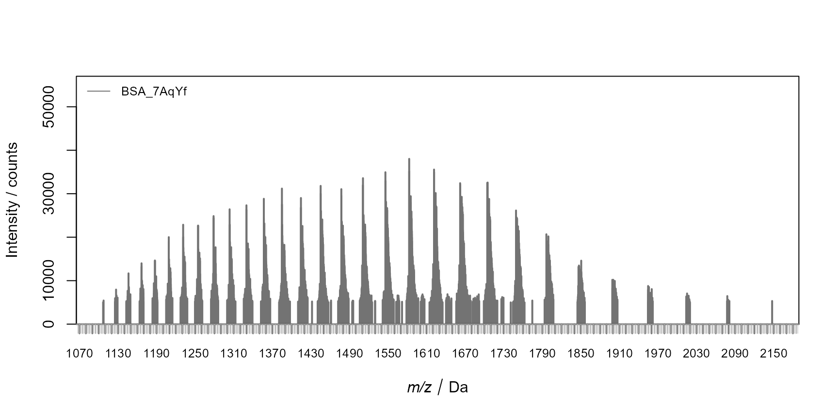
plot_spectra_charges(
ms$Results$MassSpecResults_Spectra,
colorBy = "analyses"
)Charges for the extracted spectra.
plot_spectra(ms$Results$MassSpecResults_Spectra, colorBy = "replicates")Deconvoluted and pre-processed spectra for each analysis.
Raman
The four different BSA products were measured using an online coupling of size exclusion chromatography (SEC) with capillary-enhanced Raman spectroscopy (CERS) through a liquid-core optical fiber flow cell, as reported by Thissen et al. (DOI: 10.1021/acs.analchem.3c03991). The raw spectra was converted to asc format for each retention time. A subset of the background and the main BSA elution peak was selected for pre-processing.
# Raw asc data from Raman spectroscopy
basename(raman_files)[1] "BSA_7AqYf_Raman.asc" "BSA_m595c_Raman.asc" "BSA_utpLV_Raman.asc"
[4] "BSA_wAgwS_Raman.asc"
raman <- RamanEngine$new(
metadata = list(name = "BSA Quality Evaluation Raman Project"),
analyses = raman_files
)
# Modifying the replicate names to match the MS analyses
raman$Analyses <- set_replicate_names(
raman$Analyses,
unique(get_replicate_names(ms$Analyses))[1:4]
)
DT::datatable(
info(raman$Analyses)
)
plot_chromatograms(
raman$Analyses,
yLab = "Abbundance sum for each spectrum",
colorBy = "analyses"
)Time series chromatogram for each BSA product. Each data point is a Raman spectrum at a specific retention time.
plot_spectra(raman$Analyses, rt = c(430, 440), colorBy = "analyses")Raw averaged Raman spectra for each BSA product between 430 and 440 seconds.
As for MS data, the workflow for Raman data is also assembled using an ordered list of ProcessingStep objects.
raman_workflow <- list(
RamanMethod_BinScans_native(
mode = c("time"),
value = 20
),
RamanMethod_SubtractScansSection_native(
sectionWindow = c(50, 180)
),
RamanMethod_DeleteSpectraSection_native(
min = -100,
max = 315
),
RamanMethod_SmoothSpectra_savgol(
fl = 11,
forder = 2,
dorder = 0
),
RamanMethod_DeleteSpectraSection_native(
min = 315,
max = 330
),
RamanMethod_DeleteSpectraSection_native(
min = 2300,
max = 2600
),
RamanMethod_CorrectSpectraBaseline_baseline_als(
lambda = 3,
p = 0.015,
maxit = 10
),
RamanMethod_DeleteScansSection_native(
min = 0,
max = 435
),
RamanMethod_DeleteScansSection_native(
min = 445,
max = 900
),
RamanMethod_AverageSpectra_native(
by = "replicates"
),
RamanMethod_NormalizeSpectra_minmax(),
RamanMethod_NormalizeSpectra_blockweight()
)
raman$Workflow <- Workflow(raman_workflow)
show(raman$Workflow)1: BinScans (native)
2: SubtractScansSection (native)
3: DeleteSpectraSection (native)
4: SmoothSpectra (savgol)
5: DeleteSpectraSection (native)
6: DeleteSpectraSection (native)
7: CorrectSpectraBaseline (baseline_als)
8: DeleteScansSection (native)
9: DeleteScansSection (native)
10: AverageSpectra (native)
11: NormalizeSpectra (minmax)
12: NormalizeSpectra (blockweight)A particularity of the workflow for Raman data is that the background
subtraction (workflow step number 2) is performed from a time region
(i.e., between 50 and 180 seconds) before the main BSA peak, which is
from approximately from 420 to 460 seconds. The workflow is then applied
using the run_workflow() method.
raman$run_workflow()
plot_spectra_baseline(raman$Analyses, colorBy = "replicates")Baseline correction for each spectra.
plot_spectra(raman$Analyses, colorBy = "replicates")Processed Raman spectra for each BSA product.
Fusion
The fusion of MS and Raman data is performed by combining the processed data from both engines. The data is then merged into a single data frame for statistical evaluation using a StatisticEngine, as shown in the next chapter.
ms_mat <- get_spectra_matrix(ms$Results[["MassSpecResults_Spectra"]])
raman_mat <- get_spectra_matrix(raman$Analyses)
fused_mat <- cbind(ms_mat, raman_mat)
attr(fused_mat, "xaxis.name") = "Keys"
attr(fused_mat, "xaxis.values") = seq_len(ncol(fused_mat))
str(fused_mat) num [1:4, 1:931] 0.00305 0 0.0074 0.00784 0.00284 ...
- attr(*, "dimnames")=List of 2
..$ : chr [1:4] "BSA_7AqYf" "BSA_m595c" "BSA_utpLV" "BSA_wAgwS"
..$ : chr [1:931] "363-65555" "363-65575" "363-65595" "363-65615" ...
- attr(*, "xaxis.name")= chr "Keys"
- attr(*, "xaxis.values")= int [1:931] 1 2 3 4 5 6 7 8 9 10 ...Statistic analysis
Statistic analysis is performed with the StatisticEngine for evaluation of the differences between the BSA products.
PCA
The fused data is used to create a PCA model within the StatisticEngine via a processing method based on the mdatools package.
stat <- StatisticEngine$new(
metadata = list(name = "BSA Quality Evaluation PCA Project"),
analyses = fused_mat
)
# Plots the data from the added fused data.frame/matrix
plot_data(stat$Analyses)
# Note that scale is set to FALSE to avoid scaling the data
# as block weight normalization was applied for each dataset
stat$run(
StatisticMethod_MakeModel_pca_mdatools(
center = TRUE,
ncomp = 2,
alpha = 0.05,
gamma = 0.02
)
)
summary(stat$Results$StatisticResults_PCA_mdatools$model) # summary method is from mdatools Length Class Mode
center 931 -none- numeric
scale 1 -none- logical
loadings 1862 -none- numeric
eigenvals 2 -none- numeric
method 1 -none- character
ncomp 1 -none- numeric
ncomp.selected 1 -none- numeric
info 1 -none- character
call 14 -none- call
res 1 -none- list
calres 10 pcares list
limParams 2 -none- list
T2lim 8 -none- numeric
Qlim 8 -none- numeric
alpha 1 -none- numeric
gamma 1 -none- numeric
lim.type 1 -none- character
plot_overview(stat$Results$StatisticResults_PCA_mdatools)Overview plot for the PCA model.
# Adds a color key to the loadings plot to evaluate the contribution of each dataset (i.e., MS and Raman)
plot_loadings(
stat$Results$StatisticResults_PCA_mdatools,
colorKey = rep(c("MS", "Raman"), c(ncol(ms_mat), ncol(raman_mat)))
)PCA loadings plot for the fused data.
# The mdatools S3 class model object is obtained via the active binding of the StatisticEngine
plot(stat$Results$StatisticResults_PCA_mdatools$model, show.labels = TRUE) # plot method from mdatools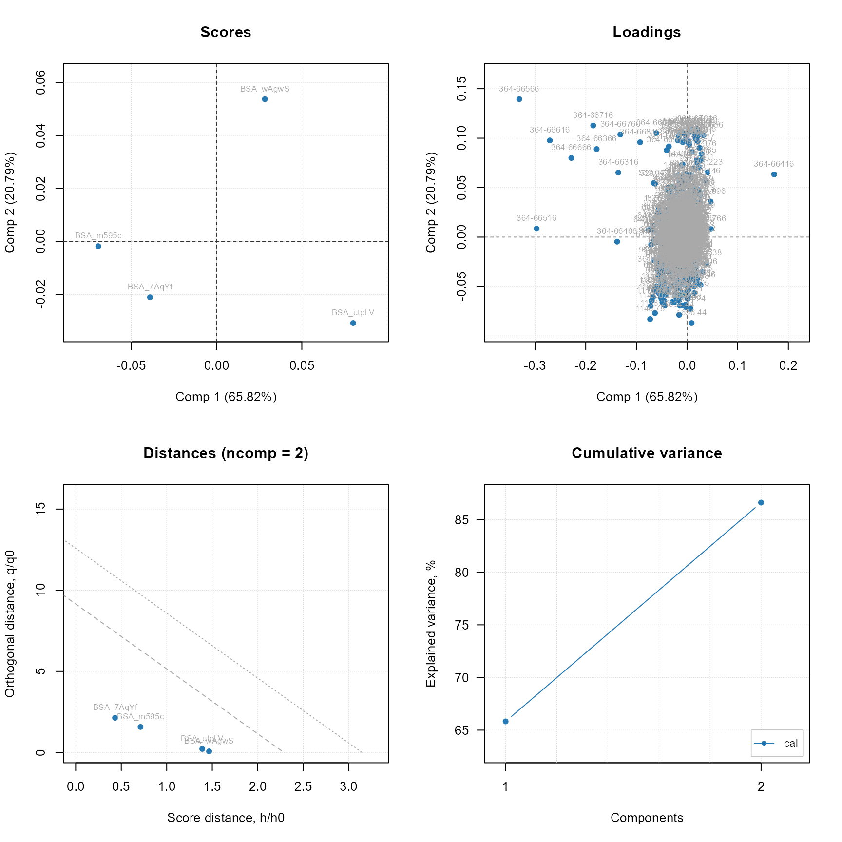
PCA summary plot using the original mdatools R package.
MCR purity
An alternative approach for the statistic analysis is the MCR pure model (also based on the mdatools R package) to evaluate the purity level of the BSA products.
stat2 <- StatisticEngine$new(
metadata = list(name = "BSA Quality Evaluation MCR Pure Project"),
analyses = fused_mat
)
stat2$run(StatisticMethod_MakeModel_mcrpure_mdatools(ncomp = 1, offset = 0.05))
summary(stat2$Results$StatisticResults_MCRPURE_mdatools$model)
Summary for MCR Purity case (class mcrpure)
Expvar Cumexpvar Varindex Purity
Comp 1 95.94 95.94 44 41.669
plot_overview(stat2$Results$StatisticResults_MCRPURE_mdatools)Overview plot of the MCR pure model.
# Gets the most pure feature for the component
get_model_data(stat2$Results$StatisticResults_MCRPURE_mdatools)$purity vars vals feature result
<int> <num> <char> <char>
1: 44 41.66906 363-66415 model