StreamFind General Introduction

The StreamFind R package is a data processing workflow designer. Besides data processing, the platform can also be used for data management, visualization and reporting. This guide focuses on describing the general framework behind StreamFind. The StreamFind is centered around R6 classes, serving as data processing engines (used as metaphor) for different types of data (e.g. mass spectrometry (MS) and Raman spectroscopy data).

Data processing engines

Data processing engines are fundamentally reference classes with methods to manage, process, visualize and report data within a project. The CoreEngine is the parent class of all other data specific engines (e.g. MassSpecEngine and RamanEngine). As parent, the CoreEngine manages the project information via the class ProjectHeaders, registers the audit trail, and contains uniform functions across child data dedicated engines (e.g. adding and removing analyses from the project).

core <- CoreEngine$new()

core


CoreEngine
name          NA
author        NA
file          NA
date          2024-08-01 10:06:20.248648

Workflow empty 

Analyses empty 

Results empty

Note that when an empty CoreEngine is created, required ProjectHeaders are created with name, author, path and date. Yet, ProjectHeaders can be specified directly during creation of the CoreEngine via the argument headers or added to the engine as shown in @ref(project-headers). The CoreEngine does not directly handle data processing. Processing methods are data specific and therefore, are used via the data dedicated engines. Yet, the framework to manage the data processing workflow and the results are implemented in the CoreEngine and are therefore, harmonized across engines.

Project headers

The ProjectHeaders S3 class is meant to hold project information that can be used to identify the engine when for example, combining different engines, or to add extra information, such as description, location, etc. The user can add any kind of attribute but it must have length one and be named. Below, ProjectHeaders are created and added to the CoreEngine.

headers <- ProjectHeaders(
  name = "Project Example", 
  author = "Person Name", 
  description = "Example of project headers"
)

core$add_headers(headers)

core$get_headers()


  ProjectHeaders 
  name: Project Example
  author: Person Name
  description: Example of project headers
  file: NA
  date: 2024-08-01 10:06:20.327951

ProcessingSettings

Data processing workflows in StreamFind are assembled by combining different processing methods in a specific order. Each processing method uses a specific algorithm for processing/transforming data at a given stage of the workflow. Thus, to harmonize the diversity of processing methods and algorithms available, a general ProcessingSettings is used (shown below). This way, the ProcessingSettings objects are use as instructions to assemble a data processing workflow within an engine.

ProcessingSettings()


 ProcessingSettings 
 engine       NA
 call         NA
 algorithm    NA
 version      0.2.0
 software     NA
 developer    NA
 contact      NA
 link         NA
 doi          NA

 parameters: empty

A ProcessingSettings object must always have the engine type, the call name of the processing method, the name of the algorithm to be used, the origin software, the main developer name and contact as well as a link to further information and the DOI, when available. Lastly but not least, the parameters which is a flexible list of conditions to apply the algorithm during data processing. As example, ProcessingSettings for centroiding MS data using the qCentroids from the qAlgorihtms and for annotating features using a native algorithm from StreamFind are shown below. Each ProcessingSettings object has a dedicated constructor method with documentation to support the usage. Help pages for processing methods can be obtained with the native R function ? or help().

MassSpecSettings_CentroidSpectra_qCentroids()


 ProcessingSettings 
 engine       MassSpec
 call         CentroidSpectra
 algorithm    qCentroids
 version      0.2.0
 software     qAlgorithms
 developer    Gerrit Renner
 contact      gerrit.renner@uni-due.de
 link         https://github.com/odea-project/qAlgorithms
 doi          https://doi.org/10.1007/s00216-022-04224-y

 parameters: 
  -  maxScale 5 
  -  mode 1

MassSpecSettings_AnnotateFeatures_StreamFind()


 ProcessingSettings 
 engine       MassSpec
 call         AnnotateFeatures
 algorithm    StreamFind
 version      0.2.0
 software     StreamFind
 developer    Ricardo Cunha
 contact      cunha@iuta.de
 link         https://odea-project.github.io/StreamFind
 doi          NA

 parameters: 
  -  maxIsotopes 5 
  -  elements C H N O S Cl Br 
  -  mode small molecules 
  -  maxCharge 1 
  -  rtWindowAlignment 0.3 
  -  maxGaps 1

Saving and loading

The CoreEngine also holds the functionality to save the project in the engine (as a SQLite file) and load it back. The save() method saves the project and the load() method loads it, as shown below.

project_file_path <- file.path(getwd(), "/project.sqlite")
core$save(project_file_path)

file.exists(project_file_path)

[1] TRUE

new_core <- CoreEngine$new()
new_core$load(project_file_path)

# The headers are has the core object although a new_core object was created with default headers
new_core$get_headers()


  ProjectHeaders 
  name: Project Example
  author: Person Name
  description: Example of project headers
  date: 2024-08-01 10:06:20.327951
  file: C:/Users/apoli/Documents/github/StreamFind/vignettes/articles//project.sqlite

Data specific engines

As above mentioned, the CoreEngine does not handle data processing directly. The data processing is delegated to child engines. A simple example is given below by creating a child RamanEngine and accessing the spectra from the analyses (added as full paths to .asc files on disk). Note that the workflow and results are still empty, as no data processing methods were applied.

# Example raman .asc files
raman_ex_files <- StreamFindData::get_raman_file_paths()
raman <- RamanEngine$new(raman_ex_files)
raman


RamanEngine
name          NA
author        NA
file          NA
date          2024-08-01 10:06:21.050755

Workflow empty 

Analyses
                         analysis                     replicate  blank spectra
                           <char>                        <char> <char>   <num>
 1:       raman_Bevacizumab_11731       raman_Bevacizumab_11731   <NA>       1
 2:       raman_Bevacizumab_11732       raman_Bevacizumab_11732   <NA>       1
 3:       raman_Bevacizumab_11733       raman_Bevacizumab_11733   <NA>       1
 4:       raman_Bevacizumab_11734       raman_Bevacizumab_11734   <NA>       1
 5:       raman_Bevacizumab_11735       raman_Bevacizumab_11735   <NA>       1
 6:       raman_Bevacizumab_11736       raman_Bevacizumab_11736   <NA>       1
 7:       raman_Bevacizumab_11737       raman_Bevacizumab_11737   <NA>       1
 8:       raman_Bevacizumab_11738       raman_Bevacizumab_11738   <NA>       1
 9:       raman_Bevacizumab_11739       raman_Bevacizumab_11739   <NA>       1
10:       raman_Bevacizumab_11740       raman_Bevacizumab_11740   <NA>       1
11:       raman_Bevacizumab_11741       raman_Bevacizumab_11741   <NA>       1
12: raman_blank_Bevacizumab_10005 raman_blank_Bevacizumab_10005   <NA>       1
13: raman_blank_Bevacizumab_10006 raman_blank_Bevacizumab_10006   <NA>       1
14: raman_blank_Bevacizumab_10007 raman_blank_Bevacizumab_10007   <NA>       1
15: raman_blank_Bevacizumab_10008 raman_blank_Bevacizumab_10008   <NA>       1
16: raman_blank_Bevacizumab_10009 raman_blank_Bevacizumab_10009   <NA>       1
17: raman_blank_Bevacizumab_10010 raman_blank_Bevacizumab_10010   <NA>       1
18: raman_blank_Bevacizumab_10011 raman_blank_Bevacizumab_10011   <NA>       1
19: raman_blank_Bevacizumab_10012 raman_blank_Bevacizumab_10012   <NA>       1
20: raman_blank_Bevacizumab_10013 raman_blank_Bevacizumab_10013   <NA>       1
21: raman_blank_Bevacizumab_10014 raman_blank_Bevacizumab_10014   <NA>       1
22: raman_blank_Bevacizumab_10015 raman_blank_Bevacizumab_10015   <NA>       1
                         analysis                     replicate  blank spectra
    traces
     <num>
 1:   1024
 2:   1024
 3:   1024
 4:   1024
 5:   1024
 6:   1024
 7:   1024
 8:   1024
 9:   1024
10:   1024
11:   1024
12:   1024
13:   1024
14:   1024
15:   1024
16:   1024
17:   1024
18:   1024
19:   1024
20:   1024
21:   1024
22:   1024
    traces

Results empty

# setting interactive to TRUE, plotly is used for an interactive plot
raman$plot_spectra(interactive = FALSE)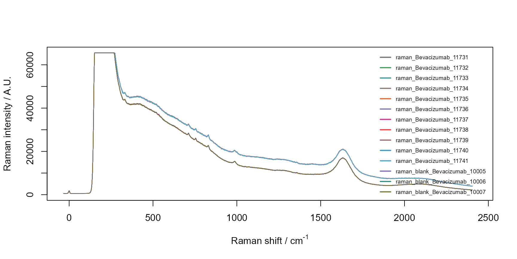

Editing analyses set

For data processing, the analysis replicate names and the correspondent blank analysis replicates can be assigned with dedicated methods, as shown below. For instance, the replicate names are used for averaging the spectra in correspondent analyses and the assigned blanks are used for background subtraction, as shown below in @ref(data-processing).

raman$add_replicate_names(c(rep("Sample", 11), rep("Blank", 11)))
raman$add_blank_names(rep("Blank", 22))

# The replicate names are modified and the blanks are assigned
raman


RamanEngine
name          NA
author        NA
file          NA
date          2024-08-01 10:06:21.050755

Workflow empty 

Analyses
                         analysis replicate  blank spectra traces
                           <char>    <char> <char>   <num>  <num>
 1:       raman_Bevacizumab_11731    Sample  Blank       1   1024
 2:       raman_Bevacizumab_11732    Sample  Blank       1   1024
 3:       raman_Bevacizumab_11733    Sample  Blank       1   1024
 4:       raman_Bevacizumab_11734    Sample  Blank       1   1024
 5:       raman_Bevacizumab_11735    Sample  Blank       1   1024
 6:       raman_Bevacizumab_11736    Sample  Blank       1   1024
 7:       raman_Bevacizumab_11737    Sample  Blank       1   1024
 8:       raman_Bevacizumab_11738    Sample  Blank       1   1024
 9:       raman_Bevacizumab_11739    Sample  Blank       1   1024
10:       raman_Bevacizumab_11740    Sample  Blank       1   1024
11:       raman_Bevacizumab_11741    Sample  Blank       1   1024
12: raman_blank_Bevacizumab_10005     Blank  Blank       1   1024
13: raman_blank_Bevacizumab_10006     Blank  Blank       1   1024
14: raman_blank_Bevacizumab_10007     Blank  Blank       1   1024
15: raman_blank_Bevacizumab_10008     Blank  Blank       1   1024
16: raman_blank_Bevacizumab_10009     Blank  Blank       1   1024
17: raman_blank_Bevacizumab_10010     Blank  Blank       1   1024
18: raman_blank_Bevacizumab_10011     Blank  Blank       1   1024
19: raman_blank_Bevacizumab_10012     Blank  Blank       1   1024
20: raman_blank_Bevacizumab_10013     Blank  Blank       1   1024
21: raman_blank_Bevacizumab_10014     Blank  Blank       1   1024
22: raman_blank_Bevacizumab_10015     Blank  Blank       1   1024
                         analysis replicate  blank spectra traces

Results empty

raman$plot_spectra(interactive = FALSE, colorBy = "replicates")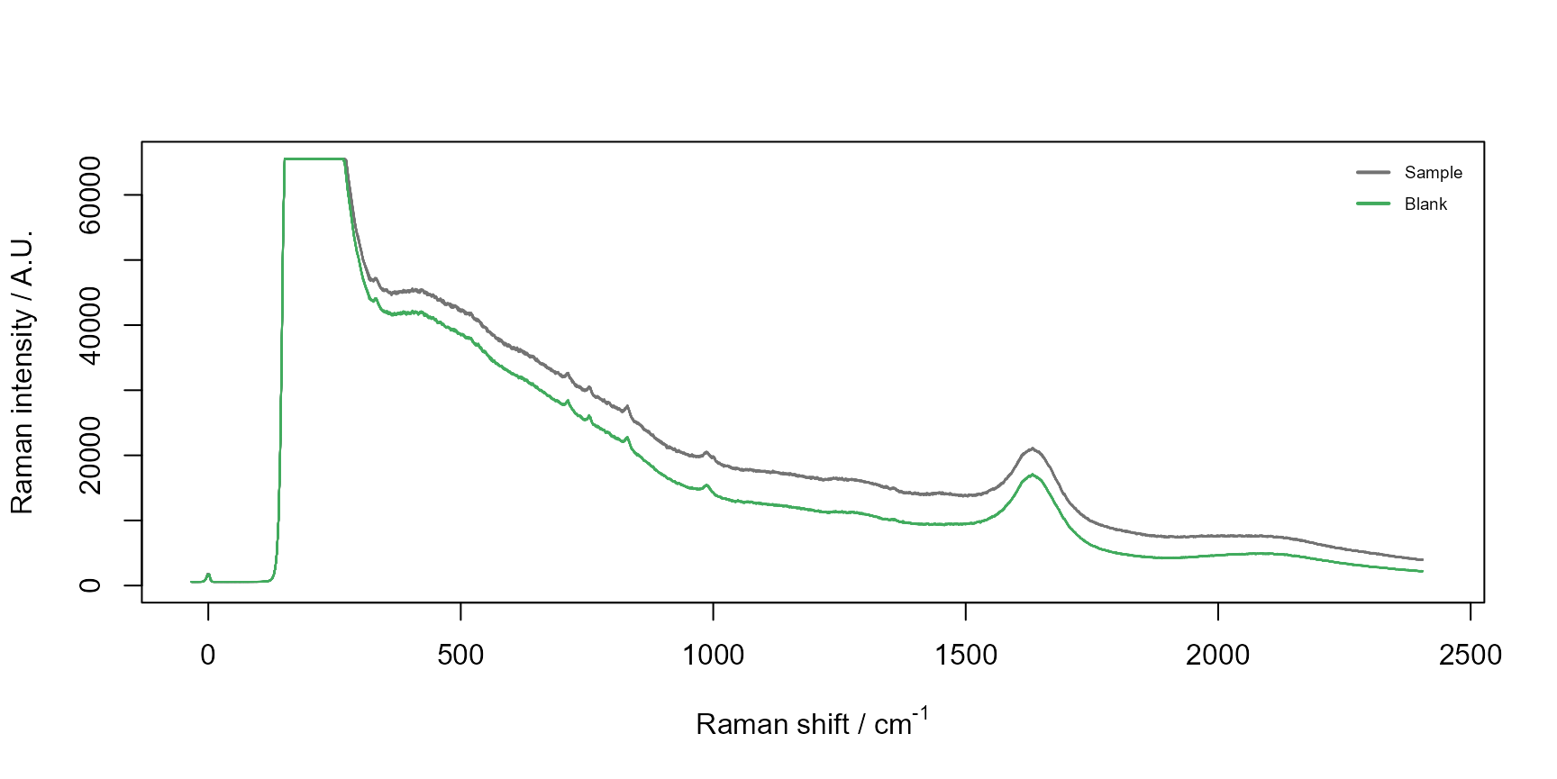

Data processing workflow

As above mentioned, ProcessingSettings are used to design an ordered data processing workflow. Below we create a simple list of ProcessingSettings for processing the Raman spectra.

ps <- list(
  # Averages the spectra for each analysis replicate
  RamanSettings_AverageSpectra_StreamFind(),
  
  # Simple normalization based on maximum intensity
  RamanSettings_NormalizeSpectra_minmax(),
  
  # Background subtraction
  RamanSettings_SubtractBlankSpectra_StreamFind(),
  
  # Applies smoothing based on moving average
  RamanSettings_SmoothSpectra_movingaverage(windowSize = 4),
  
  # Removes a section from the spectra from -40 to 470
  RamanSettings_DeleteSpectraSection_StreamFind(list("shift" = c(-40, 300))),
  
  # Removes a section from the spectra from -40 to 470
  RamanSettings_DeleteSpectraSection_StreamFind(list("shift" = c(2000, 3000))),
 
  # Performs baseline correction 
  RamanSettings_CorrectSpectraBaseline_baseline(method = "als", args = list(lambda = 3, p = 0.06, maxit = 10)),
  
  # Performs again normalization using minimum and maximum
  RamanSettings_NormalizeSpectra_minmax()
)

# The settings are added to the engine but not yet applied
raman$add_settings(ps)

raman$print_workflow()


Workflow
 1: AverageSpectra (StreamFind)
 2: NormalizeSpectra (minmax)
 3: SubtractBlankSpectra (StreamFind)
 4: SmoothSpectra (movingaverage)
 5: DeleteSpectraSection (StreamFind)
 6: DeleteSpectraSection (StreamFind)
 7: CorrectSpectraBaseline (baseline)
 8: NormalizeSpectra (minmax)

# The data processing workflow is applied
raman$run_workflow()

Results

Once the data processing methods are applied, the results can be accessed with the get_results() method.

# The spectra results is added after processing the Raman spectra 
raman


RamanEngine
name          NA
author        NA
file          NA
date          2024-08-01 10:06:21.050755

Workflow
 1: AverageSpectra (StreamFind)
 2: NormalizeSpectra (minmax)
 3: SubtractBlankSpectra (StreamFind)
 4: SmoothSpectra (movingaverage)
 5: DeleteSpectraSection (StreamFind)
 6: DeleteSpectraSection (StreamFind)
 7: CorrectSpectraBaseline (baseline)
 8: NormalizeSpectra (minmax)

Analyses
                         analysis replicate  blank spectra traces
                           <char>    <char> <char>   <num>  <num>
 1:       raman_Bevacizumab_11731    Sample  Blank       1   1024
 2:       raman_Bevacizumab_11732    Sample  Blank       1   1024
 3:       raman_Bevacizumab_11733    Sample  Blank       1   1024
 4:       raman_Bevacizumab_11734    Sample  Blank       1   1024
 5:       raman_Bevacizumab_11735    Sample  Blank       1   1024
 6:       raman_Bevacizumab_11736    Sample  Blank       1   1024
 7:       raman_Bevacizumab_11737    Sample  Blank       1   1024
 8:       raman_Bevacizumab_11738    Sample  Blank       1   1024
 9:       raman_Bevacizumab_11739    Sample  Blank       1   1024
10:       raman_Bevacizumab_11740    Sample  Blank       1   1024
11:       raman_Bevacizumab_11741    Sample  Blank       1   1024
12: raman_blank_Bevacizumab_10005     Blank  Blank       1   1024
13: raman_blank_Bevacizumab_10006     Blank  Blank       1   1024
14: raman_blank_Bevacizumab_10007     Blank  Blank       1   1024
15: raman_blank_Bevacizumab_10008     Blank  Blank       1   1024
16: raman_blank_Bevacizumab_10009     Blank  Blank       1   1024
17: raman_blank_Bevacizumab_10010     Blank  Blank       1   1024
18: raman_blank_Bevacizumab_10011     Blank  Blank       1   1024
19: raman_blank_Bevacizumab_10012     Blank  Blank       1   1024
20: raman_blank_Bevacizumab_10013     Blank  Blank       1   1024
21: raman_blank_Bevacizumab_10014     Blank  Blank       1   1024
22: raman_blank_Bevacizumab_10015     Blank  Blank       1   1024
                         analysis replicate  blank spectra traces

Results
 1: spectra

# The structure of the spectra results
str(raman$get_results("spectra"))

List of 1
 $ spectra:List of 2
  ..$ Blank :List of 1
  .. ..$ spectra:Classes 'data.table' and 'data.frame': 0 obs. of  0 variables
  .. .. ..- attr(*, ".internal.selfref")=<externalptr> 
  ..$ Sample:List of 1
  .. ..$ spectra:Classes 'data.table' and 'data.frame': 690 obs. of  6 variables:
  .. .. ..$ replicate: chr [1:690] "Sample" "Sample" "Sample" "Sample" ...
  .. .. ..$ shift    : num [1:690] 300 303 306 309 312 ...
  .. .. ..$ intensity: num [1:690] 0.0886 0.0386 0.1075 0.1457 0.2491 ...
  .. .. ..$ blank    : num [1:690] 0.75 0.733 0.717 0.706 0.695 ...
  .. .. ..$ baseline : num [1:690] 0.0454 0.0456 0.0458 0.0461 0.0463 ...
  .. .. ..$ raw      : num [1:690] 0.0452 0.0453 0.0458 0.0461 0.0467 ...
  .. .. ..- attr(*, ".internal.selfref")=<externalptr>

# Averaged spectra can be obtained with the dedicated field
raman$spectra

$Blank
Null data.table (0 rows and 0 cols)

$Sample
     replicate     shift  intensity      blank   baseline        raw
        <char>     <num>      <num>      <num>      <num>      <num>
  1:    Sample  300.2333 0.08860028 0.74995276 0.04535583 0.04520539
  2:    Sample  303.2319 0.03860228 0.73266994 0.04560113 0.04528911
  3:    Sample  306.2275 0.10750530 0.71749096 0.04584628 0.04575694
  4:    Sample  309.2201 0.14567355 0.70615152 0.04609087 0.04612487
  5:    Sample  312.2137 0.24908625 0.69497025 0.04633435 0.04670256
 ---                                                                
686:    Sample 1990.7185 0.13597257 0.06158937 0.04635464 0.04635729
687:    Sample 1992.6790 0.13359305 0.06209468 0.04625501 0.04624998
688:    Sample 1994.6373 0.12759965 0.06210308 0.04615509 0.04613068
689:    Sample 1996.5951 0.11742477 0.06252161 0.04605499 0.04599770
690:    Sample 1998.5507 0.11607689 0.06278336 0.04595484 0.04589319

# Modified spectra which results in a single spectrum
raman$plot_spectra()

Conclusion

This quick guide introduced the general framework behind StreamFind. The StreamFind is a data processing workflow designer that uses R6 classes to manage, process, visualize and report data within a project. The CoreEngine is the parent class of all other data specific engines and manages the project information via the class ProjectHeaders. The ProcessingSettings are used to harmonize the diversity of processing methods and algorithms available. The data processing is delegated to child engines, such as the RamanEngine and MassSpecEngine. The data processing workflow is assembled by combining different processing methods in a specific order. The results can be accessed with the get_results() method or dedicated methods (e.g. spectra and plot_spectra). StreamFind can also be used via the embedded shiny app for a graphical user interface. See the StreamFind App Guide for more information.

Ricardo Cunha

01 August, 2024